Space

Introduction

To avoid reinventing the wheel, the proposed data-cleaning workflow uses functions for other existing packages. In this module, we used one test of the bdc and other tests of the R package CoordinateCleaner to flag potentially erroneous, suspect, or imprecise geographical coordinates based on geographic gazetteers and metadata. It includes a series of tests for identifying records assigned to capitals, provinces, and country centroids, coordinates in urban areas, around biodiversity institutions, or GBIF headquarters. It also contains tests to flag coordinates below a determined precision (e.g., 100 km), zero or equal coordinates, and duplicated records (i.e., equal taxa name and coordinates).

Note that we do not use the “seas” test to remove records in the ocean because such records we previously removed in the pre-filter module of the package (more details here).

⚠️IMPORTANT:

The results of the VALIDATION test used to flag data quality are appended in separate fields in this database and retrieved as TRUE (✅ ok) or FALSE (❌check carefully).

Installation

Check here how to install the bdc package.

Reading the database

Reading the database created in the taxonomy module the bdc package. It is also possible to read any datasets containing the required fields to run the function (more details here).

database <-
  readr::read_csv(here::here("Output/Intermediate/02_taxonomy_database.csv"))

Flagging common spatial issues

This function identifyes records with a coordinate precision below a specified number of decimal places. For example, the precision of a coordinate with 1 decimal place is 11.132 km at the equator, i.e., the scale of a large city.

check_space <-
  bdc_coordinates_precision(
    data = database,
    lon = "decimalLongitude",
    lat = "decimalLatitude",
    ndec = c(0, 1) # number of decimals to be tested
  )
#> bdc_coordinates_precision:
#> Flagged 2 records
#> One column was added to the database.

Next, we will flag common spatial issues using functions of the package CoordinateCleaner.

check_space <-
  CoordinateCleaner::clean_coordinates(
    x =  check_space,
    lon = "decimalLongitude",
    lat = "decimalLatitude",
    species = "scientificName",
    countries = ,
    tests = c(
      "capitals",     # records within 2km around country and province centroids
      "centroids",    # records within 1km of capitals centroids
      "duplicates",   # duplicated records
      "equal",        # records with equal coordinates
      "gbif",         # records within 1 degree (~111km) of GBIF headsquare
      "institutions", # records within 100m of zoo and herbaria
      "outliers",     # outliers
      "zeros",        # records with coordinates 0,0
      "urban"         # records within urban areas
    ),
    capitals_rad = 2000,
    centroids_rad = 1000,
    centroids_detail = "both", # test both country and province centroids
    inst_rad = 100, # remove zoo and herbaria within 100m
    outliers_method = "quantile",
    outliers_mtp = 5,
    outliers_td = 1000,
    outliers_size = 10,
    range_rad = 0,
    zeros_rad = 0.5,
    capitals_ref = NULL,
    centroids_ref = NULL,
    country_ref = NULL,
    country_refcol = "countryCode",
    inst_ref = NULL,
    range_ref = NULL,
    # seas_ref = continent_border,
    # seas_scale = 110,
    urban_ref = NULL,
    value = "spatialvalid" # result of tests are appended in separate columns
  )
#> Testing coordinate validity
#> Flagged 0 records.
#> Testing equal lat/lon
#> Flagged 0 records.
#> Testing zero coordinates
#> Flagged 0 records.
#> Testing country capitals
#> Flagged 0 records.
#> Testing country centroids
#> Flagged 0 records.
#> Testing urban areas
#> Downloading urban areas via rnaturalearth
#> trying URL 'http://www.naturalearthdata.com/http//www.naturalearthdata.com/download/50m/cultural/ne_50m_urban_areas.zip'
#> Content type 'application/zip' length 452644 bytes (442 KB)
#> downloaded 442 KB
#>
#> OGR data source with driver: ESRI Shapefile
#> Source: "C:\Users\Bruno R. Ribeiro\AppData\Local\Temp\RtmpCo3Lyf", layer: "ne_50m_urban_areas"
#> with 2143 features
#> It has 4 fields
#> Integer64 fields read as strings:  scalerank
#> Flagged 6 records.
#> Testing geographic outliers
#> Testing GBIF headquarters, flagging records around Copenhagen
#> Flagged 0 records.
#> Testing biodiversity institutions
#> Flagged 0 records.
#> Testing duplicates
#> Flagged 0 records.
#> Flagged 6 of 115 records, EQ = 0.05.

Here we update the column named .summary summing up the results of all tests. This column is FALSE if any test was flagged as “FALSE” (❌check carefully; potentially invalid or suspect record).

check_space <- bdc_summary_col(data = check_space)
#> Column '.summary' already exist. It will be updated
#>
#> bdc_summary_col:
#> Flagged 9 records.
#> One column was added to the database.

Mapping spatial errors

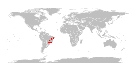
It is possible to map a column containing the results of one spatial test each time, for example records in country centroids (column “.cen”). Besides, we can use the column “.summary” to map all records flagged as potentially problematic (i.e., FALSE).

check_space %>%
  dplyr::filter(.summary == FALSE) %>% # map only records flagged as FALSE
  bdc_quickmap(
    data = .,
    lon = "decimalLongitude",
    lat = "decimalLatitude",
    col_to_map = ".summary",
    size = 0.9
  )

Records flagged as potentially problematic

Report

Creating a report summarizing the results of all tests. The report can be automatically saved if save_report = TRUE.

report <-
  bdc_create_report(data = check_space,
                    database_id = "database_id",
                    workflow_step = "space",
                    save_report = FALSE)

report

Figures

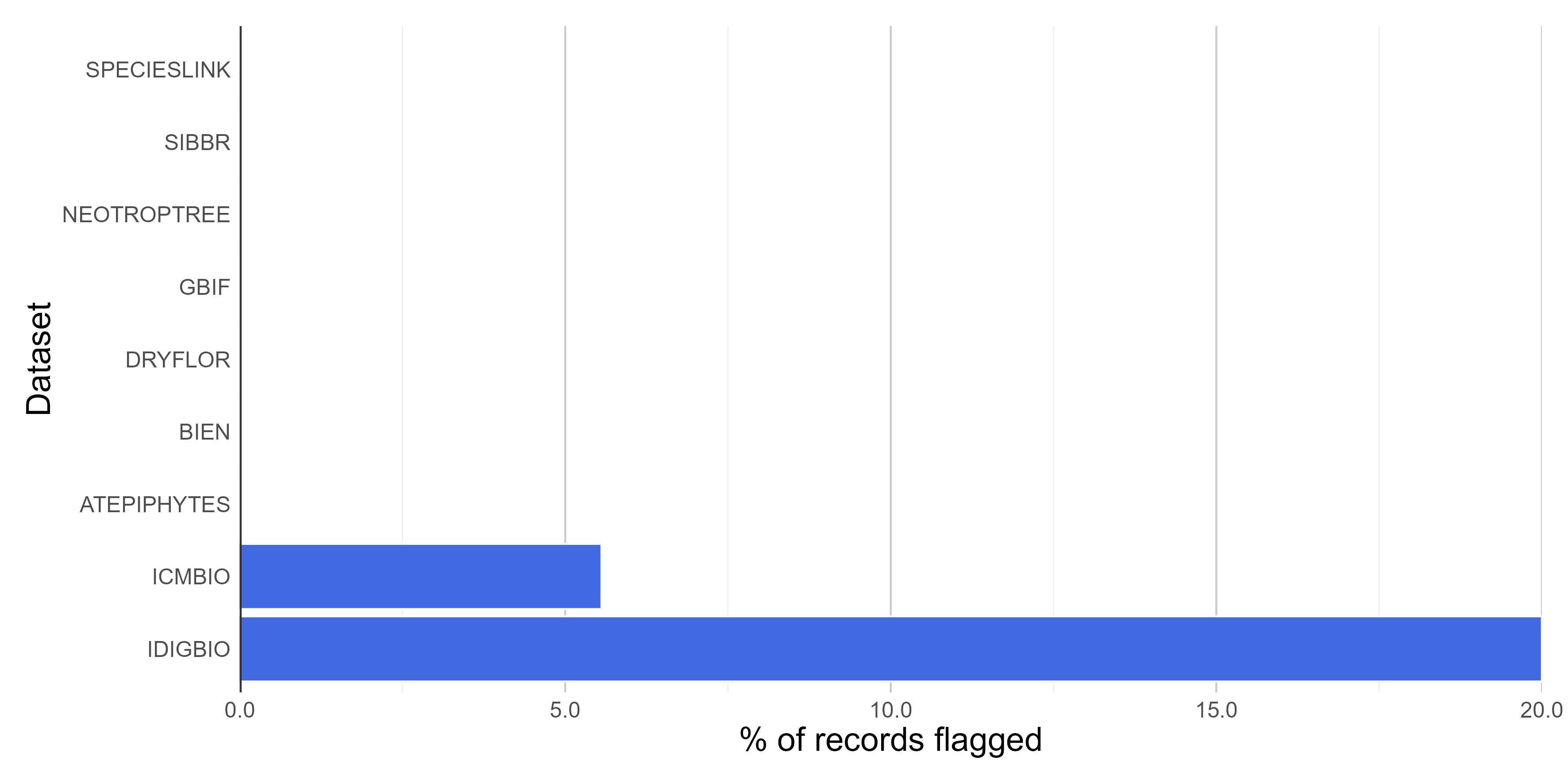
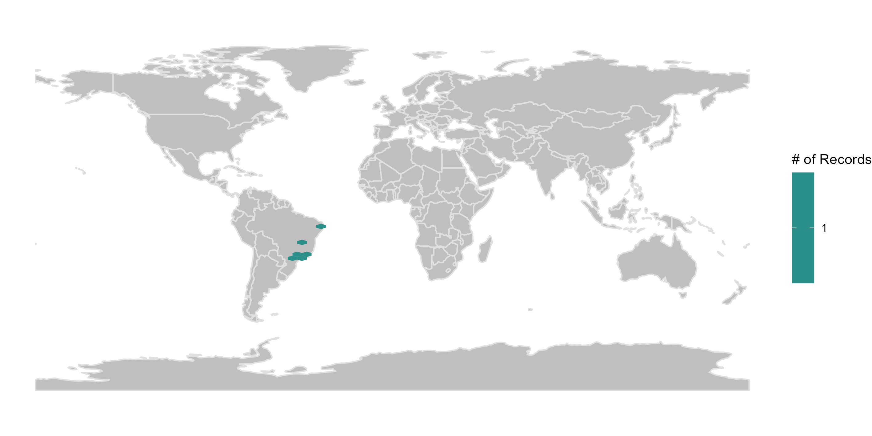
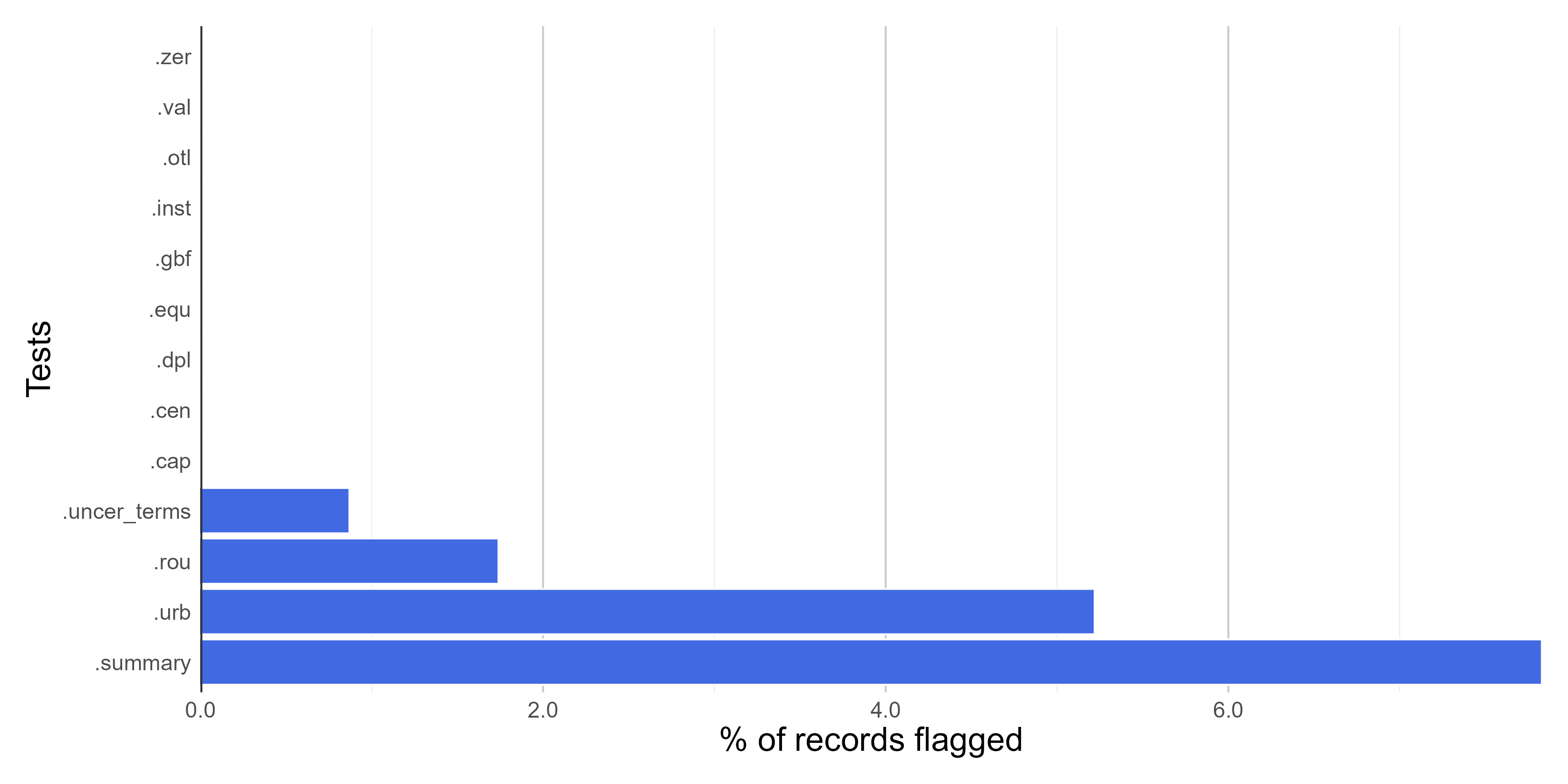
Here we create figures (bar plots, maps, and histograms) to make the interpretation of the results of data quality tests easier. Figures can be automatically saved if save_figures = TRUE.

figures <-
bdc_create_figures(data = check_space,
                   database_id = "database_id",
                   workflow_step = "space",
                   save_figures = TRUE)

# Check figures using
figures$.rou

Rounded coordinates

Records within urban areas

Summary of all tests

Filtering the database

It is possible to remove flagged records (potentially problematic ones) to get a ‘clean’ database (i.e., without test columns starting with “.”). However, to ensure that all records will be evaluated in all the data quality tests (i.e., tests of the taxonomic, spatial, and temporal module of the package), potentially erroneous or suspect records will be removed in the final module of the package.

# output <-
#   check_space %>%
#   dplyr::filter(.summary == TRUE) %>%
#   bdc_filter_out_flags(data = ., col_to_remove = "all")

Saving the database

You can use qs::qsave() instead of write_csv to save a large database in a compressed format.

# use qs::qsave() to save the database in a compressed format and then qs:qread() to load the database
check_space %>%
 readr::write_csv(.,
            here::here("Output", "Intermediate", "03_space_database.csv"))

2024-12-18